Introduction
Protein solubility and the formation of intrinsic protein particles is the focus of many biotechnological, biochemical and medical applications such as the expression and purification of therapeutic proteins, the pharmaceutical development of highly concentrated protein formulations for subcutaneous application, or the pathogenicity and appearance of different diseases (like Alzheimer’s or Parkinson’s) [1].
Therefore, improving protein solubility and circumventing colloidal instability of protein solutions and avoiding the formation of intrinsic protein particles is of upmost importance [2]. Different strategies should be considered, depending on the development stage of the respective biologic: (i) biochemical optimization of the amino acid sequence composition and/or (ii) optimization of solution conditions allowing an improvement of colloidal protein properties. Besides these strategies, a number of efforts are undertaken for the improvement of tools and algorithms for predicting protein solubility, based on the biochemical composition of the protein. Thus, at each development stage of biologics, the challenge with protein solubility has to be considered. A selection of recent advances addressing techniques for the improvement of protein solubility are discussed and evaluated.
The term solubility/insolubility is often related to the formation of intrinsic protein particles/aggregates [2]. However, there is a mechanistic difference between the two aspects. In the case of a pure solubility issue, i.e. a protein becomes insoluble in a certain solution (no changes in protein structure and integrity) and a solid phase is formed, a strong dilution of the system may lead to the dissolution of the protein. In such a circumstance, the term “protein associates” may more appropriately describe the formed protein solid [2]. In this instance, protein particles are formed, especially protein aggregates and often such aggregates cannot be dissolved by a dilution step. The reason for the formed aggregates is typically related to a perturbation of the protein structure, protein integrity, and/or chemical modification. A selection of recent techniques for the improvement of protein solubility are discussed and evaluated.
Protein Solubility
What is Solubility?
Solubility is a physicochemical property of a solid compound (alternatively a liquid or a gas), denoted as the solute, that dissolves in a liquid solvent forming a homogeneous solution of the solute in the solvent [3]. The solubility of a compound depends on the used solvent as well as temperature, pressure and the presence of excipients. The term insolubility is often applied to poorly or very poorly soluble compounds. Under certain conditions (e.g. temperature) the equilibrium solubility can be exceeded to give a so-called supersaturated solution. Such supersaturated solutions are thermodynamically metastable. From a molecular point of view, solubility can also be seen as a dynamic equilibrium process, i.e. a simultaneous process of dissolution and solid phase formation. Solubility equilibrium is reached when these two processes have the same constant rate [3]. Dissolution and solid phase formation of a compound are determined by balancing properties of various intermolecular forces between the solvent and the solute as well as the change in entropy accompanying solute solvation. All factors influencing this balance impact solubility [4, 5]. For pure solubility issues, a pure dilution step should allow the re-dissolution of the formed protein solid.
Thermodynamic Definition of Protein Solubility
From a thermodynamic standpoint, the phase (p) of a system at equilibrium is clearly defined by the variables’ temperature, pressure and composition [3]. The Gibb’s phase rule, which is only valid to systems at equilibrium, determines the number of degrees of freedom (f) in terms of state variables as: p + f = b + 2, with b the number of components. During a solubility test, the temperature and pressure are usually held constant, the Gibbs phase rule is simplified to: p + f’ = b, with f’ = f - 2 [3]. Let us consider a three component system, composed of water (solvent, denoted by an index 1), a solute (protein, denoted by an index 2) and an excipient dissolved in water (e.g. sugar, denoted by an index 3). In this case, only one solution phase is present and two degrees of freedom (f’) are available. This implicates the variation of the protein and excipient, without influencing the phase state of the solution. However, in the presence of two phases, (i.e. the appearance of a precipitate from the solution, with both phases in coexistence), and keeping the concentration of the excipient constant, f’ becomes zero. This implies that the composition of both phases must be fixed. In other words, the protein concentration in the solution phase becomes independent of the total amount of protein added to the system. A further addition of protein to the solution is not increasing the protein concentration in solution, but induces an increase of the solid phase, i.e. more protein precipitate (the solid phase) is formed (see Figure 1) according to the Gibbs phase rule [3]. At these specific conditions, protein solubility is determined (Figure 1). 
For two phases, like a solid (s) phase and a liquid (l) phase in equilibrium, the chemical potentials (μ) of the individual components (j) in the two phases are equal: μj(l) = μj(s).
When μ of the solute (2), in our case the protein, exceeds the μ of the solid phase, i.e. μ2(l) > μ2(s), protein precipitation is observed [3]. For the case of protein molecules dissolved in pure water (w) and in a solution (solution = water in the presence of an excipient) that are in equilibrium with the protein in the same solid phase, the chemical potentials of the protein in the different phases are equal: μ2(l) = μ2(l,w) = μ2(s). The term μ2(l,w) refers to protein dissolved in pure water, whereas μ2(l) relates to protein solution in an aqueous solution containing a third component (e.g. an excipient like sugar). The relation between the chemical potential and protein activity (a) in a specific phase (denoted by i) is: μ2(i) = μ2(i,0) + R·T ln a(i), with a = c·γ and c = concentration, γ = activity coefficient and μ2(i,0) = the chemical standard potential [6]. The difference between the chemical potentials of the protein in an aqueous solution and water phase is Δμ2(l) = μ2(l) - μ2(l,w) = μ2(l,0) - μ2(l,0,w) = R·T ln [c2(l,w) / c2(l)] + R·T ln [γ2(l,w)/ γ2(l)]. c2(l) and γ2(l) refer to the concentration and activity coefficient in the saturated aqueous solution, respectively. The term Δμ2(l) expresses the differences in the Gibbs free energy, which is related to protein-solvent interactions in the absence and presence of the excipient (component 3). Δμ2(l) therefore describes the transfer free energy of protein molecules from a pure water phase to an aqueous solution containing the excipient and thus the parameter Δμ2(l) is directly related to the protein solubility difference in both solvents, with the assumption that γ2(l,w) / γ2(l) equals one [4]. The above defined thermodynamic solubility implies that μ2(s) is independent of the composition of solvent in equilibrium with that solid phase [3, 4]. This assumption is valid for crystals of small molecules. However, for macromolecules like proteins, it is observed that protein crystals contain considerable amounts of water and small molecules (e.g. excipients) [4], and consequently there is a difference between the chemical potentials of the protein in solid phases in equilibrium with different aqueous solvents. In addition to this, one has to remember that μ2(s) depends on the solid state, whether a crystalline or amorphous phase is formed [7]. In a number of cases it was observed that protein solubility is much higher when the precipitated protein forms an amorphous phase compared to the formation of a crystalline phase. This indicates μ2(s,crystalline) < μ2(s,amorphous).
Based on the defined thermodynamic solubility and the consideration to apply the Gibbs phase rule to solubility data, it is indispensable to measure the solubility of the compound as a function of varying quantities of the solid phase. However, this is not always feasible [4]. Depending on the analyzed systems, the solubility curves are different (Figure 1). In Figure 1, a solubility curve is shown originating from a single protein component (curve 1), in which the composition of both phases remains constant. Solubility is given by S1. For a solid solution composed of two or more protein components, the shape of the solubility curves differs (curve 2 in Figure 1). In the case of a protein mixture composed of two proteins, the solubility curve shows two distinct breaks due to the appearance of two solid phases (curve 3 in Figure 1). However, in each of the three presented cases, the solubility becomes constant when an excess of the solid phase is present.
Kinetic versus Thermodynamic Solubility
Depending on how the solubility is measured, one distinguishes between kinetic and thermodynamic solubility Figure 2 [7]. 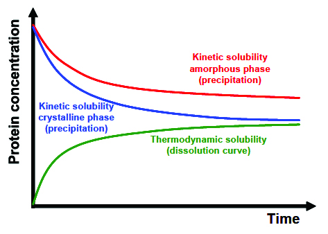 Kinetic solubility answers the extent to which a compound precipitates when added to a new solvent and how much of the compound stays in solution. Such experiments are performed by dissolving the compound in a specific solvent and pipetting it into particular buffer systems. After a certain equilibration time and phase separation step, the concentration of the compound in the tested buffer is determined [7]. Thermodynamic solubility determines how much of a compound dissolves, i.e. transfer from a solid to a liquid phase, and what concentration is reached in a specific solvent under specific environmental conditions (see chapter: Thermodynamic definition of protein solubility). In a number of cases it is observed that kinetic solubility is higher compared to thermodynamic solubility as precipitates typically form an amorphous solid phase and not a crystalline solid phase [7].
Factors Affecting Solubility
For protein solutions, one has to consider certain special conditions that may affect protein solubility [8-11]. Protein solubility is affected by native (correctly folded) protein-protein interactions. Partially denatured and especially fully denaturated proteins with increased hydrophobicity, show a much more reduced solubility compared to the native form. In most cases, the formation of denaturated proteins induces a strong increase of the solution turbidity, which is accompanied by the formation of protein particles [2, 12, 13]. Therefore, it is important to differentiate whether changes in protein solubility may be due to conformational and/or colloidal protein instabilities. The strategies to stabilize such solutions are quite different. From a biochemical point of view, protein solubility depends on the amino acid sequence composition and on the exposure of specific amino acids to the protein surface/water interface (see below). However, from a colloidal and physicochemical perspective, protein solubility depends on factors like solvent properties, solvent polarity, presence of excipients, or temperature [14]. The physical forces influencing protein solubility are electrostatic interactions, ion bridges, ion binding, hydrogen bondings, solvation and hydration properties, protonation degree, dispersion forces, osmotic pressure, hydrophobic interactions and, with this, protein-solvent, protein-excipient and/or protein-protein interactions [9, 15]. Excipients may differently (direct or indirect) interact with proteins and also may interact with different protein states (e.g. native, partially denatured or fully denatured states). The amino acid arginine is often described to improve protein solubility, especially during the purification process [16]. Nakakido et al. [17] have explained the arginine effect by a thermodynamic description. ArgHCl interacts favorably with a majority of amino acid side chains, even if binding of ArgHCl to the protein surface is limited, perhaps transient and weak. The applied Gap theory (a statistical-mechanical model of the effect of solution additives on protein association reactions) provides a kinetic aspect of ArgHCl properties, namely a destabilization of the transition state of the aggregation reaction, although the stability of the native and denatured proteins remains unchanged [17].
Improvement of protein solubility and colloidal stability of e.g. monoclonal antibodies in the presence of detergents like polysorbates is not based on specific protein-excipient interactions, but more likely on circumventing protein denaturation at the water/air interface [18, 19]. The solution hydrogen ion activity strongly influences protein solubility. In general, protein solubility becomes minimal at hydrogen ion activities close to the pK-value of the protein. The presence of ions also impacts protein solubility. The terms salting-in/ salting-out are related to the presence of certain ions that may decrease/increase protein solubility [4, 10].
No general rules are currently available for clearly manipulating and improving protein solubility; a case-by-case investigation is usually necessary.
Measuring Protein Solubility
 The direct measurement of protein solubility is challenging due to a number of issues. One problem results from the formation of gels when the protein concentration is strongly increased: no phase separation due to protein precipitation is observed. With increasing protein concentrations, highly viscous solutions (“honey-like” solution) are observed, depending on the solution conditions. Another concern is related to the fact that protein may partially or fully denature, and thus a precipitate is formed (aggregate formation). This phenomenon is not always directly related to the solubility of the native protein form. Furthermore, most solubility tests are time consuming and require large quantities (up to grams depending on the target protein concentration, which for antibodies can reach a few hundreds of milligram per milliliter) of homogeneous protein samples. Indirect techniques like the determination of the so-called osmotic second virial coefficient (B22) demonstrated to be a useful method for the selection of solution conditions showing promising solubility conditions (see below) [20-23]. The methods used for the measurement of protein solubility have been presented recently [11]. In short, these methods can be classified as follows: (i) addition of lyophilized protein to a solution until the solution becomes saturated and the solubility is reached, (ii) concentration by ultrafiltration, and (iii) protein precipitation induced by precipitants (Figure 3). Some of these techniques were described many years ago. The first relevant description of protein solubility with respect to salts as precipitants (Figure 3) was published nearly a century ago [24] and it took about 50 years for the presentation of a theoretical-based model to explain the mechanism [8]. Melander and Horvath related protein solubility to hydrophobic effects [8]. Especially polyethylene glycol (PEG) has been used as a precipitant for the determination of protein solubility [25], because a log-linear relationship between protein solubility and PEG concentration (cPEG)could be demonstrated. However, the application using PEG as precipitant for the estimation of protein solubility is only valid under certain assumptions, as described below (Figure 4A).
A general expression for the activity coefficient γ of the protein in the presence of the precipitant is given by: log γ = log γ0 + A11·S + A12·cPEG + B11·S2 + + B12· c2PEG + …, with γ0 the protein activity coefficient in dilute solution, A and B constant parameters characteristic of each term.
For dilute solutions γ0à 1, thus log γ0 = 0. All higher order terms are neglected when it can be assumed that protein-protein and PEG-PEG interactions are negligible, for quite high PEG concentrations [6]. Thus, the simplified approximation becomes: log S = log S0 - A12·cPEG, with S the solubility in the presence of PEG precipitant at a concentration cPEG. S0 is the apparent intrinsic solubility/activity obtained by extrapolation to cPEG = 0 for the protein in equilibrium with the PEG-induced precipitated protein solid phase. Thus, the presented equation is only valid for dilute solution.
As presented by Middaugh et al. (1979) [6] the form of this solubility (= activity for the activity coefficient = 1) is dependent on the choice of concentration scale and standard state, but the relationship log S = log S0 - A12·cPEG should be valid independent of this choice. If the assumption of diluted solution conditions, i.e. ideal behavior is not valid, higher order terms (e.g. B11, B12) should produce a curvature of the log S versus cPEG plots as shown in (Figure 4B, curve c4). Mechanistically, the reason for protein precipitation in the presence of PEG is due to the excluded volume effect [26-28].
For certain proteins, like deoxyhemoglobulin S, oxyhemoglobulin A or bovine serum albumin, the above described linear relationship between log S and cPEG has been demonstrated (Figure 4A) [6]. Furthermore, for these proteins, the extrapolated solubility values are independent of the total protein concentration, i.e. the curve extrapolation to cPEG = 0 for curves generated at different total protein concentrations (c1 to c3) gives one extrapolated solubility value. The above derived equations also predict a regular increase in the curve slope with increasing the protein concentration (Figure 4A) [6]. However, for a number of cases like beta-lactoglobulin or therapeutic monoclonal antibodies, these findings were not observed. A variation of the total protein concentration lead to curves with largely varying intercepts for extrapolating the curved to cPEG = 0 (Figure 4B). Thus, estimation for protein solubility is not always achievable. Moreover, nonlinearity of the curve has been observed, which is related to protein systems showing self-association properties. Thus, the PEG precipitation assay, especially in the simplified log-linear relationship, cannot be seen as an universal method for the estimation of protein solubility, and one has to be aware of the thermodynamic assumptions that justify the described data analysis. For more details see the following references: 6, 11, 25-29.
Protein Solubility and Colloidal
Solution Properties
The osmotic second virial coefficient (B22) is a parameter derived from statistical mechanics to relate the thermodynamics of solutions to the properties of the molecules that compose them, i.e. B22 measures the non-ideal solution behavior arising from two body interactions. It was shown that B22of diluted protein solutions correlates with B22 of concentrated protein solutions [23]. Therefore, B22 measurements can be realized under diluted conditions and are representative of concentrated protein solutions. The parameter B22 reflects the extent and direction of the non-ideal solution property, and thus protein-protein interactions.
Positive B22 values are indicative for solution conditions favoring the repulsion between protein molecules, whereas solution conditions with negative B22 values show attractive protein properties that support the formation of protein precipitates. Various studies showed the osmotic second virial coefficient as a valuable parameter for the optimization of crystallization solution conditions (BB22 < 0, usually between -1 and -8·10-4 mol·ml·g-2) [5, 22, 23 and references cited therein].
The aim using the osmotic second virial coefficients is the determination of the strength of protein-protein interactions via B22, which is used for the identification of solution conditions minimizing protein-protein interactions.
There are two main methods to determine B22, namely static light scattering and self-interaction chromatography (SIC) (for more details see Lebrun et al. [21] and references cited therein).
In SIC, the protein of interest is covalently bound to chromatography particles and the retention volume of aqueous protein solutions injected in the chromatography column is measured. The retention volume of the protein depends on the interaction between the free protein in solution and the protein bound to the chromatography particles. B22 is calculated using the retention volume [21, 22]. The osmotic second virial coefficient is correlated with protein solubility [30], and the data show that B22 is a useful parameter for the identification of solution conditions maximizing protein solubility. Table 1 summarizes the relative solubility of an enzyme as a function of pH. Solution conditions with a positive B22 show much higher protein solubility compared to solution conditions with negative B22 values.
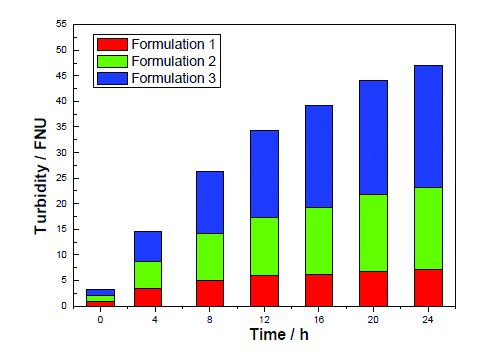 Besides solubility, colloidal stability is also increased for solution conditions with positive B22 values (Figure 5). Colloidal stability was assessed in a stirring experiment, where the protein solution was extensively stirred [14, 20]. The formation of protein particles, measured by turbidity, increases faster for the protein dissolved in a solution (Figure 5, formulation 3) with B22 < 0.
Especially the use of automated chromatography equipment makes SIC a valuable method for the rational screening of solution conditions improving protein solubility. As an indirect method, the concept of investigating the osmotic second virial coefficient allows the identification of “best solubility solution conditions”, with a probability of reaching high protein solubilities.
Protein Biochemistry and Protein Engineering
The biochemical composition of the protein amino acid sequence determines strongly the ability of a protein to dissolve in an aqueous medium and to induce the formation of aggregates [31, 32].
The current trends for the prediction of protein-protein interaction of proteins and of the identification of protein aggregation/association prone regions can be categorized as follows: (1) phenomenological models (PM) and (2) molecular simulation (MS) techniques [33]. PMs use physicochemical properties such as the hydrophobicity of the protein, and beta-sheet propensity (e.g. TANGO algorithm [34]), in order to identify aggregation prone regions from protein primary sequences. Such approaches have been successfully applied for small peptides [34] and denatured proteins. However, for larger molecules like antibodies with a more or less globular structure, the prediction of aggregation propensities might differ, because protein-protein interactions are mainly influenced by the tertiary structure and the stability of the native state.
The second approach, molecular simulation techniques (e.g. atomistic models), is based on three-dimensional structures and uses the dynamics and fluctuations of proteins to estimate the amino acid regions, which show a higher tendency to induce the formation of aggregates. The main problem using MS techniques for the investigation of large molecules results from the extremely high computer power demand.
Trout and colleagues [33, 35, 36] developed a method based on atomistic simulations of full antibody to predict antibody aggregation prone regions [34]. This method is based on the “spatial-aggregation-propensity (SAP)”, which is a parameter of the dynamic exposure of hydrophobic patches [35]. They have explored the effect of different hydrophilic mutations on these predicted aggregation prone regions to engineer antibodies with enhanced stability. Chennamsetty et al. [34] were able to show that a mutation to lysine is more effective than serine but less effective than glutamic acid in enhancing antibody stability. The same group has also investigated cysteine variants of antibodies with respect to colloidal stability [36]. In addition, they showed that multiple simultaneous mutations on different SAP peaks can have a cumulative effect on enhancing protein stability [34].
Because of economical aspects of such simulations, Trout et al. analyzed the accuracy of various cheaper alternatives for SAP evaluation. Antibody fragment (Fab, Fc) simulations, implicit solvent models, or direct computations from a static structure (i.e., a structure from X-ray or homology modelling) were identified as valuable and cheaper alternatives [34]. The last option is often not feasible during the early development phase of biologics, because X-ray structures are in most cases not available.
Their study showed that the derived SAP from a static structure, which is about 200,000 times faster, still predicts most of the major aggregation prone regions [34]. This makes it a potential approach for the use in high-throughput applications, although being less accurate compared to the SAP from explicit atomistic simulations.
Using logistic regression, Diaz et al. [37] predicted the protein solubility of proteins over-expressed in Escherichia coli, whereas Waldo [38] used genetic screens and directed evolution, in which protein diversity libraries are screened for soluble variants to understand and predict protein solubility.
Various other strategies, like sequence-based approaches, rationally designed mutations, hydrophobicity engineering or artificial neural networks have been presented [for more details see: 39-43].
Conclusions
Protein solubility and improving protein solubility are of great interest in the scientific, technical and economic communities. However, more should be known about the parameters governing protein solubility and how solubility can be manipulated in a rational way.
Understanding protein solubility in a broader sense may allow a better understanding of the causes for the appearance of certain diseases. This may also lead to more successful development of biologics by reducing the propensity of therapeutic proteins to form particles and thus improve the general safety of the drug product. Furthermore, it allows development of highly-concentrated protein formulations for e.g. subcutaneous application and economic improvement (e.g. purification and recovery) of the manufacturing process.
Significant efforts are still required to develop methods for measuring or even predicting protein solubility. As a powerful tool for a rational solubility solution screening, the approach using the osmotic second virial coefficient seems very promising.
Acknowledgements
V. Le Brun and Stefan Bassarab are acknowledged for support and fruitful discussions.
References
1. P. Garidel, S. Bassarab, “Impact of formulation design on stability and quality”, In: Lycson N (ed). Quality for biologics: critical quality attributes, process and change control, product variation, characterisation, impurites and regulatory concerns. Hamphshire: Biopharm Knowledge Publishing, 2009, 94-113.
2. P. Garidel, F. Kebbel, “Protein therapeutics and aggregates characterized by photon correlation spectroscopy”, BioProcess Int. 2010, 8 (3), 38-46.
3. G. Wedler, “Lehrbuch der Physikalischen Chemie”; 3. edition, 1987, VCH, Weinheim.
4. T. Arakawa, S. N. Timasheff, “Theory of protein solubility”, Methods Enzymol. 1985, 114, 49-77.
5. N. Asherie, “Protein crystallisation and phase diagrams”, Methods 2004, 34, 266-272.
6. C.R. Middaugh, W.A. Tisel, R.N. Haire, A. Rosenberg, “Determination of the apparent thermodynamic activities of saturated protein solutions”, J. Biol. Chem. 1979, 254, 367-370.
7. C. Saal., “Optimising the solubility of research compounds”, Am. Pharm. Rev. 2010, May/June Issue, 12-15.
8. W. Melander, C. Horvath, ”Salt effects on hydrophobic interactions in precipitation and chromatography of proteins: An interpretation of the lyotropic series”, Arch. Biochem. Biophys. 1977, 183, 200–215.
9. A. Ben-Naim, “Solvation and solubility of globular proteins”, Pure & Applied Chem. 1997, 69, 2239-2243.
10. F. Hofmeister, “Zur Lehre von der Wirkung der Salze. Zweite Mittheilung”, Archive Exp. Pathol. 1888, 24, 247-260.
11. S.R. Trevino, J.M. Scholtz, C.N. Pace, “Measuring and increasing protein solubility”, J. Pharm. Sci., 2008, 97, 4155-4166.
12. W. Wang, S. Nema, D. Teagarden, “Protein aggregation – pathway and influencing factors”, Int. J. Pharm. 2010, 390, 89-99.
13. K. Schumacher, G. Winter, H.C. Mahler, “Instability of protein drugs [Instabilitäten von Proteinarzneimitteln]”, PZ Prisma 2003, 10 (1), 15-18.
14. V. Le Brun, W. Friess, S. Bassarab, P. Garidel, “Correlation of protein-protein interactions as assessed by affinity chromatography with colloidal protein stability: A case study with lysozyme”, Pharm. Dev. Technol. 2010, 15 (4), 421-430.
15. A. Saluja, D.S. Kalonia, “Nature and consequences of protein-protein interactions in high protein solutions”, Int. J. Pharm. 2008, 358, 1-15.
16. C. Lange, R. Rudolph, “Suppression of protein aggregation by L-arginine”, Current Pharm. Biotechnol. 2009, 10 (4), 408-414.
17. M. Nakakido, M. Kudou, T. Arakawa, K. Tsumoto, “To be excluded or to bind, that is the question: arginine effects on proteins” Current Pharm. Biotechnol. 2009, 10, 415-420.
18. P. Garidel, C. Hoffmann, A. Blume, “A thermodynamic analysis of the binding interaction between polysorbate 20 and 80 with human serum albumins and immunoglobulins: A contribution to understand colloidal protein stabilisation”, Biophys. Chem. 2009, 143 (1-2), 70-78.
19. C. Hoffmann, A. Blume, I. Miller, P. Garidel, “Insights into protein-polysorbate interactions analysed by means of isothermal titration and differential scanning calorimetry”, Eur. Biophys. J. 2009, 38 (5), 557-568.
20. V. Le Brun, W. Friess, S. Bassarab, S. Mühlau, P. Garidel, “A critical evaluation of self-interaction chromatography as a predictive tool for the assessment of protein-protein interactions in protein formulation development: A case study of a therapeutic monoclonal antibody”, EJPB 2010, 75 (1), 16- 25.
21. V. Le Brun, W. Friess, T. Schultz-Fademrecht, S. Mühlau, P. Garidel, “Lysozyme-lysozyme self-interactions as assessed by the osmotic second virial coefficient: Impact for physical protein stabilization”, Biotechnol. J. 2009, 4 (9), 1305-1319.
22. P.M.Tessier, S.I. Sandler, A.M. Lenhoff, “Direct measurement of protein osmotic second virial cross coefficients by cross-interaction chromatography”, Protein Sci. 2004, 13, 1379-1390.
23. J.J. Valente, K.S. Verma, M.C. Manning, W.W. Wilson, C.S. Henry, “Second virial coefficient studies of cosolvent-induced protein self-interaction”, Biophys. J. 2005, 89, 4211-4218.
24. E.J. Cohn, “The physical chemistry of the proteins”, Physiol. Rev. 1925, 5, 349–437.
25. C.L. Stevenson, M.J. Hageman, “Estimation of recombinant bovine somatropin solubility by excluded-volume interaction with polyethylene glycols”, Pharm. Res. 1995, 12, 1671-1676.
26. D.H. Atha, K.C. Ingham, “Mechanism of precipitation of proteins by polyethylene glycols”, J. Biol. Chem. 1981, 256, 12108-12117.
27. K.C. Ingham, “Protein precipitation with polyethylene glycol”, Methods in Enzymology 1984, 1043, 351-356.
28. R.R. Burgess, “Protein precipitation techniques”, Methods in Enzymology 2009, 463, 331-342.
29. D.R.H. Evans, J.K. Romero, M. Westoby, “Concentration of proteins and removal of solutes”, Methods in Enzymology 2009, 463, 97-120.
30. S. Ruppert, S.I. Sandler, A.M. Lenhoff, “Correlation between the osmotic second virial coefficient and the solubility of proteins”, Biotechnol. Prog. 2001, 17, 182-187.
31. W.R. Taylor, A. Aszódi, “Protein geometry, classification, topology and symmetry. A computational analysis of structure”; 2005, Institute of Physics Publishing, Bristol and Philadelphia.
32. N.Tokuriki, F. Stricher, J. Schymkowitz, L. Serrano, D.S. Tawfik, “The stability effects of protein mutations appear to be universally distributed”, J. Mol. Biol. 2007, 369 (5), 1318-1332.
33. N. Chennamsetty, V. Voynov, V. Kayser, B. Helk, B.L. Trout, “Prediction of aggregation prone regions of therapeutic proteins”, J. Phys. Chem. B 2010, 114 (19), 6614-6624.
34. A.-M. Fernandez-Escamilla, F. Rousseau, J. Schymkowitz, L. Serrano, “Prediction of sequence-dependent and mutational effects on the aggregation of peptides and proteins”, Nature Biotech. 2004, 22 (10), 1302-1306.
35. N. Chennamsetty, V. Voynov, V. Kayser, B. Helk, B.L. Trout, “Design of therapeutic proteins with enhanced stability”, PNAS 2009, 106 (29), 11937- 11942.
36. V. Voynov, N. Chennamsetty, V. Kayser, H.J. Wallny, B. Helk, B.L. Trout, “Design and application of antibody cysteine variants”, Biocon. Chem. 2010, 21 (2), 385-392.
37. A.A. Diaz, E. Tomba, R. Lennarson, R. Richard, M.J. Bagajewicz, R.G. Harrison, “Prediction of protein solubility in Escherichia coli using logistic regression”, Biotech. Bioeng. 2010, 105 (2), 374-383.
38. G.S Waldo, ”Genetic screens and directed evolution for protein solubility”, Current Opin. Chem. Biol. 2003, 7 (1), 33-38.
39. M. Murby, E. Samuelsson, T.N. Nguyen, L. Mignard, U. Power, H. Binz, M. Uhlen, S. Stahl, “Hydrophobicity engineering to increase solubility and stability of a recombinant protein from respiratory syncytial virus”, Eur. J. Biochem. 1995, 230 (1), 38-44.
40. M. Malissard, E.G. Berger, “Improving the solubility of the catalytic domain of human β-1,4-galactosyltransferase 1 through rationally designed amino-acid replacements” Eur. J. Biochem. 2001, 268, 4352-5358.
41. S. Venturea, “Sequence determinants of protein aggregation: tools to increase protein solubility” Microb. Cell Factories 2005, 4, 11, 8 pages.
42. P. Smialowski, A.J. Martin-Galiano, A. Mikolajka, T. Girschick, T.A. Holak, D. Frishman, “Protein solubility: Sequence based prediction and experimental verification”, Bioinformatics 2007, 23 (19), 2536-2542.
43. S.R. Trevino, J.M. Scholtz, C.N. Pace, “Amino acid contribution to protein solubility: Asp, Glu, and Ser contribute more favorably than the other hydrophilic amino acids in RNase Sa”, J. Mol. Biol. 2007, 366 (2), 449-460.
Author Biography
Dr. Patrick Garidel studied chemistry and biotechnology at the University of Kaiserslautern, earning a Ph.D. in Physical Chemistry/Biophysics. His main interests are focused on protein biochemistry and stability, development and manufacturing of biologics, drug delivery systems, gene therapy, process development, and analytics.