Due to its simplicity and precision, laser diffraction is an analytical technique frequently used in the determination of particle size distribution profiles. For a commonly used laser diffraction instrument, the wide dynamic range is accomplished by using a sequential combination of measurements with red and blue light sources. The wide range of the instrument is also achieved using mathematical algorithms based on laser diffraction theory, such as Mie Theory. Mie Theory is a rigorous solution for the scattering from a spherical, homogeneous, isotropic and non-magnetic particle based on the properties of a collimated, monochromatic light source. This work is concerned with understanding how the instrument’s internal algorithms account for both red and blue light sources to accurately determine particle size distribution profiles. Of interest is the expected overlapping region of each light source scattering pattern of the same particle size, studied by measuring the particle size distribution of narrowly dispersed standards across the 0.300 μm to 100 μm range. The data are evaluated using non-parametric statistical methods and considering the goodness-of-fit of the results.

Introduction

Determination of particle size distribution profiles by laser diffraction is a common analytical technique utilized across multiple industries. A quick literature search results in hundreds of articles reporting on the applications of laser diffraction to measure particle size in natural sediments,1-3 combustion research4-6 and pharmacy.7-9 The versatility of the technique can be attributed to its capacity to analyze the diffracted light of an ensemble of particles, and its ability to perform measurements of wet and dry material dispersions,10,11 resulting in particle size characterization in a short period of time. Because of this, constant improvements to analytical instrumentation based on the principles of laser diffraction theory are being made to improve its accuracy and precision, as well as its analytical range. For a commonly used laser diffraction instrument in the pharmaceutical industry, the wide dynamic range is accomplished by using, “a sequential combination of measurements with red and blue light sources to measure across the entire particle size range … an advanced focal plane detector design able to resolve very small diffraction angles… and a powerful 10 mW solid state blue light source.” This wide range also is achieved using complex mathematical algorithms based on laser diffraction theory, such as Mie Theory. Mie Theory is a rigorous solution for the scattering from a spherical, homogeneous, isotropic and non-magnetic particle of any diameter in a non-absorbing medium based on the known properties of a collimated, monochromatic light source.12 Derived from Maxwell’s Equations, Mie Theory also considers the refractive and absorption indices of the material and the medium. Given the aforementioned conditions, this work seeks to understand the relationship between the two light sources used in the determination of particle size distribution profiles despite the fact Mie Theory only considers one wavelength of light as part of its mathematical framework. For the purpose of data collection, a series of 63 detectors is utilized. According to Mie Theory, diffraction light patterns vary depending on the refractive and absorption indices of the material and the medium as well as the wavelength of the light source interacting with the ensemble of particles, which would result in different signal intensities (diffraction patterns) identified by each detector. Since “a sequential combination of measurements with red and blue light sources” is employed to determine the particle size, it is reasonable to expect each channel (detector) will be populated by signals from both light sources. If so, the question remains as to how the internal algorithm combines and deconvolutes the signals when measurements are performed using both light sources and the blue light data are subtracted from the raw light energy signal. For this purpose, the expected overlapping region of each red and blue scattering light patterns of the same particle size population was studied by measuring the particle size distribution of narrowly dispersed standards chosen across the 0.1 μm to 100 μm range. Evaluation of the raw data was performed using non-parametric statistical methods and by taking into consideration the goodness-of-fit of the resulting model. These findings are expected to contribute in procuring a more cost- and time-effective approach in the design of accurate and robust particle size testing methods as part of the pharmaceutical product development process.
Materials and Methods
National Institute of Science and Technology certified narrowly dispersed polystyrene particle size standards, which were certified by the National Institute of Science and Technology in the 0.1 μm to 100 μm range, were chosen (0.300 μm, 1 μm, 10 μm and 100 μm) to ensure the expected overlapping region between the scattering patterns of both red and blue light sources was covered. Thirty measurements of the background signal were collected during the equilibration time (12 seconds per light source) using the testing parameters appropriate for polystyrene beads (Table S1). The instrument was realigned and a new background was collected immediately before addition of any standard for the first time. All background measurements were performed using both light sources. Physical properties inherent to the material, such as refractive and absorption indices, were loaded from the instrument’s internal database and verified with each standard’s certificate of analysis.
For the analysis involving all standards at once; the normalized sum of the individual experimental datasets for each standard size (collected using both light sources at the most appropriate obscuration value) was used for comparison, instead of a multimodal simulated dataset. Hence, the comparison was performed among equally weighted data sets of the same nature to understand the effect of multiple particle size distributions at once on the resulting particle size distribution profile.
Determining Appropriate Obscuration
The first phase of the study focused on determining the most appropriate obscuration value for each particle size standard to rule out variances in particle sizes due to obscuration. Thirty measurements were collected at each of the obscuration values listed in Table S2. For this portion of the study, both light sources were used.
The JMP statistical software package was used to perform a Friedman’s means comparison rank test between the different obscuration datasets per standard size.13,14 The mean comparison was performed at the 95% (p = 0.05) confidence level with n ≈ 3,000. The null hypothesis (H0) for the Friedman test is there are no differences between the means of each dataset. The critical value is given by the χ2 (Chi-Square) distribution. If the calculated probability is low (p less than 0.05 or χ2-calculated is greater than χ2-table), the null-hypothesis is rejected, and it can be concluded at least two of the means are significantly different from each other. The effect of obscuration on each experimental dataset was evaluated against the standards’ certificates of analysis specifications through the generation and inclusion of a randomly generated and normally distributed set of particle size values as part of the statistical mean comparison. These datasets (“Simulations”) were created using the JMP scripting language (JSL) under the assumption that in an ideal case scenario, the particle size distribution of each standard would be normally distributed. The mean and standard deviation values listed in each standard’s certificate of analysis were used to simulate the normal distributions (n = 3,000).
Particle size data generated by laser diffraction are presented on a volume basis. Once the light energy versus detector number signal (63 detectors) is collected, Mie Theory is utilized to transform the data into a particle size distribution profile describing the volume occupied by each particle size present in the sample population. A particle size histogram is generated by populating 100 log-spaced bins ranging from 0.01 μm to 3,500 μm. These histograms are then typically represented with a smooth curve by connecting the midpoints of each bin. Because of the binning, an otherwise continuous response is turned into a discrete one, which also influences the variance of the population, as only a finite number of discrete bins are populated in the process of generating a particle size distribution histogram.
The experimental particle size histograms were exported from the instrument and rebinned by taking the average of two bin limits in the raw data (midpoint) and reassigning the datapoints accordingly.
This was done to minimize the difference between the particle size histograms plotted within JMP and the particle size curves reported by the instrument. Once the data were rebinned, the counts within each set of 30 measurements were added (equivalent to 30 observations of the same dispersion per obscuration value) and the corresponding histogram was generated using a JSL script.

Given the distribution differences between the simulated (continuous) and the experimental particle size data (discrete due to binning), and including their unequal variances, Friedman’s Rank Test was necessary to statistically compare the means of each population. Friedman’s test does not require the data to be neither only continuous nor only discrete, and the typical assumptions of normality and homoscedasticity do not apply. Friedman’s test does require; however, the datasets to be: 1) equal in size (accomplished by removing a handful of counts from the bin with the highest frequency in each set); and 2) block-centered.
As a result of block-centering the data, the variances of each population are transformed. This is particularly evident for the simulated datasets, for which the distribution of their datapoints is broadened when the calculation of the block means take place. The block means are calculated by taking the average of the datapoints belonging to the same block (rank) within each dataset. Nevertheless, useful information regarding binning frequency and the distribution of the experimental data within each set relative to each other can be obtained, as the block-centered data allows for a descriptive representation of the weight of each bin value. The appropriate obscuration values for each particle size standard were determined using the (Mean-Mean0)/Std0 value resulting from the Friedman’s Rank Test and the goodness-off-fit of the particle size data. The most appropriate obscuration value had to: 1) have a (Mean-Mean0)/Std0 closest to that of the simulated standard distribution; and 2) have the least number of fi t residuals > 1.00%. In this case, given both refractive and absorption indices for polystyrene are accurate, a poor fit (residuals > 1.00%) can be attributed to low signal-to-noise ratio due to low concentration or, at the other extreme, multiple scattering.
Light Source Effect
The standards were analyzed as previously described at specific obscuration target values given in Table S2. The obscuration values were chosen based on the data collected during the first phase of the study. A 60-second premeasurement delay was allowed between the background monitoring portion and the particle size analysis. The first 30 measurements were collected using both light sources, then the blue light source was turned off (Don’t Perform Blue Light Measurement: Checked) and an additional series of 30 measurements was performed using the same dispersion. Finally, the “Remove Blue Light from Analysis” function was utilized to reprocess the first set of 30 measurements and “subtract” the blue light data.
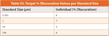
Upon analysis of each individual particle size standard, the light source effect was evaluated in the same manner for all standard sizes present at once. The approximate amount of standard-added equivalent to each obscuration target is listed in Table S3. The overall obscuration value was 12%. Statistical comparison of the population means was performed using Friedman’s Rank Test as described previously.
Relationship Between Particle Size Distribution Profile and Detector Signal
To understand the relationship between detector signal and particle size distribution, the sum of the detector signal of each experimental dataset for each standard size was normalized and compared to the detector signal of the analysis involving all standards at once (like the treatment given to the raw particle size histograms in the previous section). The square root of the absolute difference between each dataset was plotted against particle size bin or detector number accordingly to easily display the relationship between detector signal variance and its effect on the variance of the particle size distribution profile. The plots were generated using the JMP statistical software package.
Subscribe to our e-Newsletters
Stay up to date with the latest news, articles, and events. Plus, get special offers
from American Pharmaceutical Review – all delivered right to your inbox! Sign up now!
Results and Discussion
Figure 1 shows a representative particle size distribution profile (simulated and experimental) for the 0.300 μm particle size standard. Additional representative histograms for each standard are included in Figures S1, S2 and S3. While both the simulated and experimental histograms can be graphically fitted to a normal curve (in red), the experimental results ‘“deviate from normality“ due to discontinuity produced by the binning of the raw data, which in turn affects the homoscedasticity of the variances. Nevertheless, the experimental results are comparable to the certificate of analysis’ specifications.
Determining Appropriate Obscuration
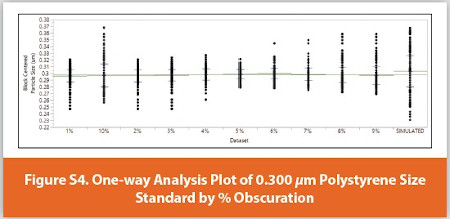
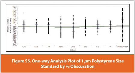
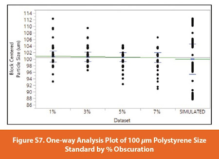
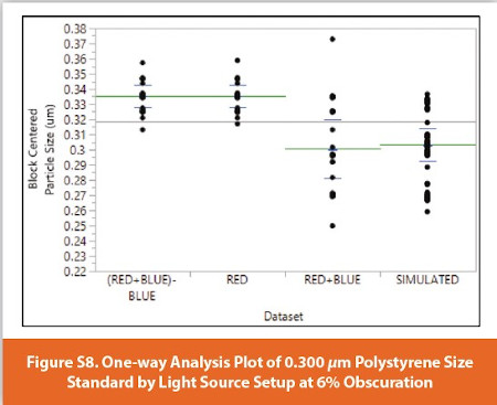
The results from the percent obscuration statistical evaluation are shown in Table 1. JMP outputs are included in Figure S4 to Figure S7, and Table S4 to Table S11. The data consist of a collection of one-way plots, means and standard deviations for each block-centered dataset and their corresponding Friedman Rank Test outputs. The one-way plots provide a visual representation of the distribution of the data within each dataset and relative to each other. One-way plots also provide a graphical representation of the means (blue) and standard deviations (green) of each set and the actual values are included in the corresponding means and standard deviations figures. In addition to their resulting (Mean-Mean0)/Std0 values, the goodness-of-fi t of each experimental dataset at each percentage obscuration value was considered to determine a stable experimental obscuration region to evaluate the effect of the red and blue light sources. This was done to establish the most appropriate experimental conditions, so any variances could be attributed to the difference in light sources utilized. Table 1 also shows the number of residuals greater than 1.00% for each dataset.
For both the 0.300 μm and 1 μm standards, datapoints tend to fall more heavily within bins located toward the upper limit of the set for lower obscuration values and primarily populate bins located toward the lower limit of the set for higher obscuration percentages. However, both standards show evenly distributed datapoints in the 5-10% range, approximately. This means within this range, the distribution of the experimental data most closely resembles a normal distribution.


Though at first glance the means of each population are practically the same despite not having equal variances, statistically, the effect of percent obscuration is still discernable. In addition to the varied distribution of the data within each set, the Friedman Rank Test output resulted in a statistically significant p-value (less than 0.05). This means at least two datasets are different from each other. In both cases, the 0.300 μm and 1 μm standards, the (Mean-Mean0)/Std0 value for the simulated datasets was the most positive (60.511 and 17.235, respectively), with values such as 2.284 (6% obscuration) and 7.335 (3% obscuration) being the closest. Those datasets with the most even distribution of data points across the range (5-10% obscuration datasets), also possess positive (Mean-Mean0)/Std0 values, which further supports the notion these are the most comparable experimental datasets to the simulated ones, generated based on the specifications listed in each standard’s certificate of analysis.
For the 10 μm and 100 μm standards, the trends are reversed. The experimental data appears more heavily weighted toward the lower particle size bins for lower obscuration values and the (Mean-Mean0)/Std0 values for the simulated datasets were the most negative. This reversal could be attributed to the fact particle sizes at this size range predominantly manifest forward scattering, whereas the diffraction patterns for the 0.300 μm and 1 μm standards are composed of significant amounts of both back and forward scattering. The effect of percentage obscuration across the test range is not as pronounced, particularly for the 10 μm standard, for which all mean values lie along the grand mean line. For this specific standard, the datasets with the most even distribution of points (6-7% obscuration) have positive (Mean-Mean0)/Std0 values, and the simulated data looks weighted toward the upper limit of the set. This could be explained by recalling each mean block is calculated by taking into consideration each point from each set that belongs to the same block (or rank). In this case, the smaller number of datasets available to compare results in a skewed weighting of the simulated datapoints. Nevertheless, the mean population values are still accurate to the raw experimental and simulated histograms. This is not the case for the 100 μm, where the simulated data are evenly distributed across the range of the dataset, as with the 0.300 μm and 1 μm standards. For each 10 μm and 100 μm standard, the most comparable datasets based on their (Mean-Mean0)/Std0 values were 1% and 7%, respectively.
Except for the 10 μm standard, there are specific percent obscuration values for which no residuals greater than 1.00% were counted, which means, at these concentrations, the signal detected by the instrument is sufficiently intense to result in an accurate fit and particle size distribution profile. The poor fit characteristic of the 10 μm particle size datasets could be attributed to its predominant forward scattering and the fact the data are collected using two light sources, though no concrete evidence was collected to support this claim.
In summary, percent obscuration values at approximately 2-7% depending on the particle size, were determined to be the most appropriate to perform the light source evaluation based on having (Mean-Mean0)/Std0 values closest to the simulated datasets and goodness-of-fit with the most residual values less than 1.00%.
Light Source Effect
Figure S8 to Figure S12 and Table S12 to Table S21 provide the results of the statistical evaluation of the effect of both light sources in the determination of particle size distribution profiles. A summary of the results can be seen in Table 2. As with the percent obscuration evaluation, the results consist of a collection of one-way plots, a list of means and standard deviations and the Friedman Rank Test output.
The effect of the light source is particularly pronounced for the 0.300 μm standard, where using the blue light source in conjunction with the red light improves the accuracy of the measurement by approximately 10%. This effect is still observable, though to a lesser extent, at the 1 μm particle size, becoming negligible for the 10 μm and 100 μm particle size standards. Based on their (Mean-Mean0)/Std0 values, the rejection of the null hypothesis can be directly attributed to the simulated dataset for the 10 μm and 100 μm standards, whereas for the 0.300 μm and 1 μm, both the simulated and the RED+BLUE datasets are significantly different from the RED and (RED+BLUE)-BLUE data. The Friedman Rank Test output shows there is no difference between the RED and (RED+BLUE)-BLUE datasets at any particle size, meaning “removing” the blue light data from the measurement has no effect on the results and the signal generated by each light source is captured within specific detector numbers (not convoluted). The red and blue light data are each directed to specific channels (1 through 51 and 52 through 63, respectively) by the instrument, and the signal intensity at these channels is not a combination of the signal produced by each light source.
When the experimental histogram corresponding to all the particle size standards in the same dispersion (“ALL” dataset) is compared against the normalized sum of the experimental histograms of each standard collected using both light sources (“COMBINED” dataset), the statistical results show a significant difference between datasets, which can be attributed to the weighting of the data across the bins. The normalized data sum results in an approximately equal weight of each particle size standard peak, as supported by the mean of the dataset [(0.300 μm + 1 μm + 10 μm + 100 μm)/4 = 27.825 μm, experimental = 23.835 μm]. This is not the case for the experimental dataset in which all standards were present at once, as the addition of the standards was not performed to result in the same volume percentage of particles per particle size standard (experimental mean ≈ 82 μm). The utilization of both light sources produced a slightly different (though practically negligible) result when compared to the RED and (RED+BLUE)-BLUE datasets. Removing the blue light data did not affect the results as well, maintaining this dataset comparable to the RED dataset. Finally, though the p-value is less than 0.05, it is “not as significant” as the previously determined p-values, which results from the comparison being performed among experimental datasets only, rather than comparing among experimental and simulated datasets.
Relationship Between Particle Size Distribution Profile and Detector Signal
In the interest of understanding the resulting difference between the ALL and COMBINED datasets, an evaluation of the light energy versus detector number and its relationship to the particle size distribution profiles was performed. Figure 2 shows an overlay of the light energy versus detector data of both the COMBINED (green = 100 μm, red = 10 μm, and magenta = 1 μm) and ALL (blue) datasets. The signal corresponding to the 0.300 μm is not sufficiently intense to be pictured in the overlay.
From Figure 2, both the location and intensity of resulting particle size distribution is a function of not only which detectors are populated, but also the intensity of the light energy signal at each detector. This is particularly illustrated with the 0.300 μm standard. A significant portion of the light energy versus detector signal for this standard is masked by the signal corresponding to the other standards. The intensity of the light energy signal is directly comparable to the intensity of the particle size peaks on a volume basis, as shown in Figure 3 and Figure 4. Furthermore, the analysis correctly identifies the presence of this particle size among all the other particles, as exemplified by the resulting particle size profile illustrated in Figure 5 (blue).
The relationship observed between the utilization of the red and blue light sources as well as light energy and particle size peak intensities can be used to develop robust particle size testing methodology. The analyst can focus on the effect of testing parameter variance on detector signal in addition to the particle size profile itself and establishing a less variable detector signal will translate into a less variable particle size distribution profile.
Figure 3 and Figure 4 illustrate the square root of the difference between the normalized ALL and COMBINED datasets, which show any differences in intensity in the particle size profile (an average of approximately 10 √μm) are equivalent to the differences observed between the detector signals (approximately 5 √arb. unit). These figures also picture the inverse relationship between detector number and particle size bin. Figure 5 shows the particle size distribution profiles from the individual determinations at the 0.300 μm (cyan), 1 m (magenta), 10 μm (red), 100 μm (green) standard sizes, and for all standards/same aliquot (blue).
Conclusions
The Friedman Rank Test and goodness-of-fit were utilized to statistically evaluate the effect of the light source setup (red light only versus red and blue) in the determination of particle size distribution profiles, as well as the relationship between both light sources. Percent obscuration values at approximately 2-7% depending on the particle size, were determined to be the most appropriate to perform the light source evaluation.
Upon conclusion of the percent obscuration value determination, the Friedman Rank Test showed a statistically significant effect of the blue light on the generation of the particle size distribution for the 0.300 μm and 1 μm size standards, for which the most accurate measurements were obtained when both light sources were used. However, this effect becomes negligible for the 10 μm and 100 μm standards. Furthermore, subtraction of the blue light source data from those experimental datasets collected using both light sources had no effect, meaning the data generated by each light source populates different detectors.
In Memoriam
In memory of Kristopher Garibay, a former PPD Laboratories employee, one of our original authors who performed much of the lab work that formed the basis of this article.
References
- Storti F, Balsamo F, Particle size distributions by laser diffraction: Sensitivity of granular matter strength to analytical operating procedures. Solid Earth. 2010; 1: 25-48. doi:10.5194/se-1-25-2010.
- Hayton S, Nelson CS, Ricketts BD, Cooke S, Wedd MW, Effect of Mica on Particle-Size Analyses Using the Laser Diffraction Technique. Journal of Sedimentary Research. 2001; 71 (3): 507–509. doi:10.1306/2dc4095b-0e47-11d7-8643000102c1865d.
- Mason JA, Greene RSB, Joeckel RM, Laser diffraction analysis of the disintegration of aeolian sedimentary aggregates in water. Catena. 2011; 87 (1):107-118. doi:10.1016/j. catena.2011.05.015.
- Black DL, McQuay MQ, Bonin MP, Laser-based techniques for particle-size measurement: A review of sizing methods and their industrial applications. Progress in Energy and Combustion Science. 1996. 22 (3): 267-306. doi:10.1016/s0360-1285(96)00008-1.
- Paulrud S, Mattsson JE, Nilsson C, Particle and handling characteristics of wood fuel powder: effects of different mills. Fuel Processing Technology. 2002. 76 (1): 23-39. doi:10.1016/s0378-3820(02)00008-5.
- Cabra R, Hamano Y, Chen JY, Dibble RW, Acosta F, Holve D, Ensemble Diffraction Measurements of Spray Combustion in a Novel Vitiated Coflow Turbulent Jet Flame Burner. NASA. 2000. WSS/CI 00S-47.
- Chew NYK, Chan H, Influence of Particle Size, Air Flow, and Inhaler Device on the Dispersion of Mannitol Powders as Aerosols. Pharmaceutical Research. 1999. 16 (7): 1098–1103. doi:10.1023/a:1018952203687.
- Zeng X, MacRitchie HB, Marriott C, Martin GP, Correlation between Inertial Impaction and Laser Diffraction Sizing Data for Aerosolized Carrier-based Dry Powder Formulations. Pharmaceutical Research. 2006. 23 (9): 2200–2209. doi:10.1007/s11095-006-9055-9.
- Chan LW, Tan LH, Heng PWS, Process Analytical Technology: Application to Particle Sizing in Spray Drying. AAPS Pharmaceutical Science Technology. 2008. 9 (1): 259–266. doi:10.1208/s12249-007-9011-y.
- Kwak B, Lee JE, Ahn J, Jeon T, Laser diffraction particle sizing by wet dispersion method for spray-dried infant formula. Journal of Food Engineering. 2009. 92 (3): 324-330. doi:10.1016/j.jfoodeng.2008.12.005.
- Li H, Seville PC, Williamson IJ, Birchall JC, The use of amino acids to enhance the aerosolisation of spray‐dried powders for pulmonary gene therapy. Journal of Gene Medicine. 2005. 7: 343-353. doi:10.1002/jgm.654.
- Mie G, Beiträge zur Optik trüber Medien, speziell kolloidaler Metallösungen. Annalen der Physik. 1908. 330: 377-445. doi:10.1002/andp.19083300302.
- JMP®, Version 14.2.0. SAS Institute Inc., Cary, NC, 1989-2019.
- Conover WJ, Practical Nonparametric Statistics. 3rd ed. Wiley; 1999. p. 367-373.