Multivariate Analysis of Cell Culture Bioprocess Data

Abstract

Multivariate time-course data generated from cell culture processes are difficult to analyze because of multicollinearity, multidimensionality, missing data and measurement uncertainty. In this study, orthogonal partial least squares regression (OPLS) analysis is used to analyze data from 21 Chinese Hamster Ovary (CHO) cell culture bioreactor batches. The parameters include temperature, pH, dissolved oxygen, viable cell density, viability, glucose, lactate etc. This multivariate method can provide insight for bioprocess development and manufacturing. It has applications in process scale-up, real-time process monitoring, process control and fault diagnosis.

Introduction

Therapeutic monoclonal antibodies are mainly expressed by recombinant Chinese Hamster Ovary (CHO) cells and are manufactured in cell culture processes. There are three unit operations in a typical cell culture process. For the first unit operation (vial thaw and flask expansion), a single frozen vial from a cell bank is thawed, and the cells are suspended in a shake flask. After a couple of days, the culture is expanded by addition of medium into another flask. This expansion method is repeated until enough inoculum exists to transfer the culture to the second unit operation. The second unit operation (seed bioreactor expansion) uses the same expansion method as the first unit operation. There are two to four seed bioreactors and each subsequent seed bioreactor is progressively larger than the previous one. The third unit operation, called production bioreactor, starts by transferring the culture from the second unit operation into a production bioreactor. The bioreactor process conditions are set to promote cell growth and production of monoclonal antibodies. Culture temperature, pH, dissolved oxygen, viable cell density, viability, glucose, lactate, and titer are monitored over time.^1-5

There are several challenges to analyze complex data generated from a cell culture process. First, the culture process variables such as pH, temperature, dissolved oxygen, glucose, and lactate are highly correlated, since they are directly related to cell growth. For example, glucose is the main energy source for antibody production while lactate is a byproduct of antibody production. In addition, there exist many missing values due to instrument issues. When ordinary least squares regression (OLS) is used to analyze cell culture process, due to correlation, the off-diagonal elements of X’X will be large and it usually results in very wide confidence intervals for the regression coefficients.

Statistical Method

In order to analyze multivariate correlated data, the Partial Least Squares or Projections to Latent Structures (PLS) method was developed by Herman Wold in the 1970s and was originally applied to econometric data.6 Assume that X denotes a n × p matrix for cell culture variables, and Y is a n × m matrix for cell culture responses, where p is the number of cell culture variables, m is the number of cell culture responses, and n is the number of cell culture observations. A typical PLS model can be written as follows:

In the X space, 1x− ’ is the variable averages and originates from the pre-process step, the matrix T is called the scores matrix that stores the maximal variation from X, the matrix P is called the loadings matrix that contains the directions of latent variables for X, and the matrix E is called the residual matrix for X. Similarly, in the Y space, 1y− ’ is the response averages and originates from the pre-process step, the matrix U is the scores matrix that stores the maximal variation from Y, the matrix C is the loadings matrix that contains the directions of latent variables for Y, and the matrix F is the residual matrix for Y. T and U are calculated to maximize the covariance between X and Y. In the PLS method, the systematic variation in the X space is divided into two parts: the systematic variability TP’ and the residual variability E. More statistical details can be found in reference 6, 7, and 8.^6-8

The PLS method has many advantages over the traditional OLS method for correlated multivariate data. PLS provides more robust estimates for highly correlated variables than OLS does, since it uses the orthogonal score matrix T to predict U, instead of just relying on the original matrix X. In addition, PLS works better for data containing missing values, because the non-linear iterative partial least squares (NIPALS) algorithm computes one column or row at a time and always converges. Due to these advantages, PLS has been successfully used in many fields, such as economics, bioinformatics, chemometrics, and statistics.^9-16

The Orthogonal Partial Least Squares (OPLS) method was developed by Johan Trygg and Svante Wold in 2002 for chemometrics.¹⁷ In the OPLS method, the systematic variation in the X space is divided into three parts: a predictive part that is correlated to Y and is designated by the subscript P, an orthogonal part that is uncorrelated to Y and is designated by the subscript O, and a residual part.^6,8,17

Data Analysis and Discussion

An OPLS batch evolution model was developed using SIMCA® 16. Viable cell density (VCD), viability, CO2, pH, O2, glucose, lactate, and sodium are treated as variables in the X space. These variables were automatically centered and scaled to unit variance by SIMCA before the analysis. Duration (day) was treated as the Y response. An OPLS model with duration as the response resulted in a three component model i.e. a predictive component and two orthogonal components. The goodness of fit measure, R2, is 0.868, indicating that the model can explain approximately 86.8% of the variation in the data. The goodness of prediction measure, Q2, is 0.974, indicating that the model predicts 97.4% of the future variation. The first component, the predictive part, explains 32.8% of the variation in the cell culture variables related to the X space. The second and the third components, the orthogonal parts, explain 38% and 16% of the variation in the cell culture variables related to the X space. Obviously, there exists a large amount orthogonal variation in the cell culture process and OPLS helps us separate the undesired orthogonal variation and focus on the predictive part of the variation that can be used to predict the response.

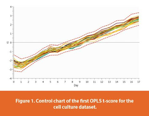
The control chart of the first OPLS t-score is shown in Figure 1. The red dash lines are the control limits, calculated as the average ± three standard deviations. All bioreactor batches behave well according to the upper and lower control limits. There is a steady trend from low scores on day zero to high scores on day seventeen.

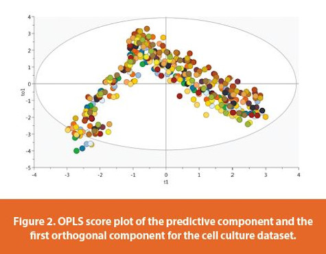
The evolution of the 21 batches of the cell culture dataset is shown in Figure 2. The horizontal axis is the predictive component t1 and the vertical axis is the first orthogonal component to1. The 95% confidence ellipse is calculated based on Hotelling’s T2 statistic and is used to find potential outliers. Since most of the dots are inside the confidence ellipse, no outliers are identified. The dots coming from the same batch are denoted with the same color. These batches behave similarly. Every batch starts in the lower left quadrant of the score plot and moves upward along the to1 direction. This trend continues until day 7, then each batch shifts to the lower right quadrant of the score plot.

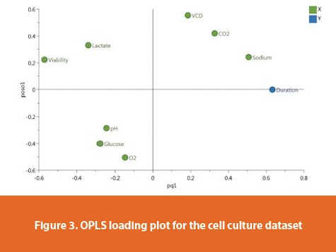
In a loading plot, the horizontal axis pq1 is the combined vector from the X loading weight p and the Y loading weight q, and the vertical axis poso1 is the combined vector from the orthogonal loading po of the X part and the projection of to onto Y so. Closed variables in the loading plot are strongly correlated. In Figure 3, viability and duration are in the opposite quadrants, indicating that they are negatively correlated. We observe that viability is usually high (around 100%) in the early stage of batch evolution and is usually low (around 60%) in the late stage of batch evolution. In addition, sodium is positively correlated to duration, because sodium is a main component of the feed and was added into the bioreactor during batch evolution.

Subscribe to our e-Newsletters
Stay up to date with the latest news, articles, and events. Plus, get special offers
from American Pharmaceutical Review – all delivered right to your inbox! Sign up now!

In order to check the influence on the response for each variable in the OPLS model, a Variable Importance in the Projection (VIP) plot is generated. It consists of three parts: VIP for the predictive part, VIP for the orthogonal part, and VIP for the total model.¹⁸ In Figure 4, all variables are ranked according to their importance to the response. Viability is the most important variable for this cell culture process and sodium is the second most important one. Interestingly, this result is consistent with what has been shown in the loading plot.

Application

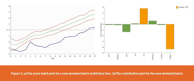
It is expensive to produce therapeutic monoclonal antibodies and the manufacturing cost for each batch can be around 3 million US dollars.¹⁰ One important application for this OPLS model is bioprocess monitoring. In Figure 5(a), a batch tunnel (as indicated by the control limits on Figure 1) is developed based on 21 batches. The green dashed line shows the batch average, and the red dashed lines show the three standard deviation control limits. It is apparent that the new batch, represented by the blue solid line, falls outside the lower control limit from day zero and never recovers. In order to understand the root cause for the deviation, we use the contribution plot to investigate why a new batch is different from the other batches in the score control chart. Figure 5(b) shows the differences for all the variables in the OPLS model between the new observation and the average observation at a given day, multiplied by the absolute value of the normalized weight.¹⁸ Here, O2 and sodium are outside the three standard deviation limits and need to be adjusted in order to bring the batch to normal conditions.

Conclusion

A large amount of data are generated from cell culture processes. The variables are usually highly correlated which makes it challenging to analyze data of this complexity. The orthogonal partial least squares method has been successfully applied to multivariate data, resulting in dimension reduction and partitioning the original data into a predictive part, an orthogonal part, and a residual part. This model can be used for bioprocess monitoring and early detection of batch deviation and is helpful to find which variables may contribute to the deviation. The expectation is that the application of the OPLS method to data of this type can be used to reduce sizeable losses due to batch failures.

References

1. California Separation Science Society (CASSS). CASSS information page. Available at: https://cdn.ymaws.com/www.casss.org/resource/resmgr/cmc_no_amer/cmc_amab_case_study/A-Mab_Case_Study_Version_2-1.pdf. Accessed March 2, 2020.
2. Sauer PW, Burky JE, Wesson MC, Sternard HD, Qu L. A high-yielding, generic fed-batch cell culture process for production of recombinant antibodies. Biotechnology and Bioengineering. 2000;67(5):585-597.
3. Heath C, Kiss R. Cell Culture Process Development: Advances in process engineering. Biotechnology Progress. 2007;23(1):46-51.
4. Zhou W, Hu W. On-line characterization of a hybridoma cell culture process. Biotechnology and Bioengineering. 1994;44(2):70-177.
5. Xing Z, Kenty BM, Li ZJ, Lee SS. Scale-up analysis for a CHO cell culture process in large-scale bioreactors. Biotechnology and Bioengineering. 2009;103 (4):733-746.
6. An Overview of Orthogonal Partial Least Squares. Available at: https://towardsdatascience.com/an-overview-of-orthogonal-partial-least-squares-dc35da55bd94. Accessed March 2, 2020.
7. 7. Introduction to Projection to Latent Structures. Available at:
8. 8. https://learnche.org/pid/latent-variable-modelling/projection-to-latent-structures/index. Accessed Mar 2, 2020
9. Eriksson L, Byrne T, Johansson E, Trygg J, Vikstrom C. Multi- and Megavariate Data Analysis: Basic Principles and Applications. 3rd ed. Malmo, Sweden: Umetrics; 2013.
10. Roychoudhury P, O’kennedy Ronan, Faulkner J, McNeil B, Harvey LM. Implementing multivariate data analysis to monitor mammalian cell culture processes. European Pharmaceutical Review. 2013;18(3):15-20.
11. Kelley B. Industrialization of mAb production technology: the bioprocessing industry at a crossroads. MAbs. 2009;1(5):443-452.
12. Abdi H. Partial least squares regression and projection on latent structure regression (PLS Regression). WIREs Computational Statistics. 2010;2(1):97-106.
13. Wold S, Antti H, Lindren F, Ohman J. Orthogonal signal correction of near-infrared spectra. Chemometrics and Intelligent Laboratory Systems. 1998;44:175-185.
14. Barker M, Rayens W. Partial least squares for discrimination. J. Chemometrics. 2003;17:166-173.
15. Haenlein M, Kaplan A. A beginner’s guide to partial least squares analysis. Understanding Statistics. 2004;3:283-297.
16. Nguyen DV, Rocke DM. Tumor classification by partial least squares using microarray gene expression data. Bioinformatics. 2002;18(1):39-50.
17. Hair JF, Sarstedt M, Hopkins L, Kuppelwieser VG. Partial least squares structural equation modeling (PLS-SEM): An emerging tool in business research. European Business Review. 2014;26(2):106-121.
18. Trygg J, Wold S. Orthogonal projections to latent structures (O-PLS). J. Chemometrics. 2002;16:119-128.
19. SIMCA User guide and tutorial, version 16, Sartorius Stedim, Umea Sweden. Acknowledgements The authors would like to thank Kristi Griffiths, William Clark, Chao Li, Anthony Maguire, Meng Zhao, Yao-ming Huang, Daniel Marasco for their advice and comments.

Author Biographies

Jinxin Gao is a principal research scientist at Eli Lilly and Company. His research is focused in statistical applications to bioproduct development. He completed his PH.D in Chemistry and Ph.D. in Statistics at University of South Carolina. Email: [email protected]

Eric Adamec is a research scientist at Eli Lilly and Company. His research is focused in statistical applications to bioproduct development. He completed his M.S in Statistics at University of Arizona. Email: [email protected]