Introduction
Multivariate analysis (MVA) is the statistical analysis of many variables at once. Many problems in the pharmaceutical industry are multivariate in nature. The importance of MVA has been recognized by the US FDA in the recent guidance on process analytical technology [1]. MVA has been made much easier with the development of inexpensive, fast computers and powerful analytical software. Chemometrics is the statistical analysis of chemical data, which is an important area of MVA. Spectral data from modern process or laboratory instruments is fundamentally multivariate in character. Furthermore, the powerful statistical methods of chemometrics are nearly essential for the analysis and application of spectral data including Near IR and Raman spectra [2]. Chemometrics has also become common in the analysis of MS and LC-MS data. There are numerous recent reviews of quantitative analysis of pharmaceutical products using MVA [2-4]. In this article, we will review several different chemometric methods for qualitative analysis. The methods, in increasing order of sensitivity, that are discussed in this paper are wavelength correlation (WC), principal component analysis (PCA), soft independent modeling of class analogies (SIMCA), and partial least squares discriminate analysis (PLS-DA).
Wavelength Correlation
The most common application of qualitative analysis with NIR and Raman data is the identification of raw and in-process materials. The standard chemometric method for identification is wavelength correlation. In wavelength correlation a test spectrum,  , is compared with a product reference spectrum,
  using a normalized vector dot product.
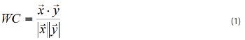
The reference spectrum can be a single spectrum or an average of several spectra. If the test spectrum is nearly identical with the reference spectrum, the wavelength correlation value is near 1.0 (e.g. 0.99). A poor match is less than 0.8. Typically a threshold of 0.95 or higher is used to identify raw materials. The wavelength correlation approach is simple and robust and is an excellent default method for identification. WC is often performed after spectral pre-processing, e.g. a first derivative. A method related to wavelength correlation is Euclidean distance. The ED parameter is the absolute value of the difference between a test and reference spectrum, given in equation 2.
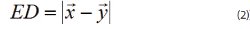
A matching spectrum will have a small Euclidean distance value (<0.1). If x and y are normalized spectrum, then the ED values are directly related to wavelength correlation.

A detailed review of raw material library validation and documentation can be found elsewhere [3].
PCA
An important method for qualitative analysis of spectral data is PCA, principal component analysis. PCA is a method for the investigation of the variation within a multivariable data set. The first step in PCA is to subtract the average value or spectrum from the entire data set, this is called mean centering. The largest source of variation in the data set is called principal component (PC) 1. The 2nd largest source of variation in the data, which is independent of PC 1, is called PC 2. Principal components form a set of orthogonal vectors. For each one of the data points, the projection of the data point onto the P1 or P2 vector is called a score value. Plots of sample score values for different principal components, typically P1 versus P2 are called score plots. Score plots provide important information about how different samples are related to each other. Principal component plots, also called loading plots, provide information about how different variables are related to each other.
The mathematics of PCA can be clearly described using linear algebra [5]. An excellent discussion of linear algebra can be found in reference [6]. By convention, the data matrix, X, has p columns and n rows, and each column represents another variable and new rows for each observation or sample. The average data matrix, , is the average of each individual column (i.e. variable) in the data set.Mean centering is written as

The covariance matrix is written as

Where an upper script T represents a matrix transpose. The covariance matrix is a square, symmetric, p x p matrix. The covariance matrix provides information about the relationship between different variables. For example, the i,j element of the covariance matrix quantifies the relative change between the i,j variables. If an element of the covariance matrix is zero, there is no relationship (correlation) between the two variables. Related to the covariance matrix is the correlation matrix where all the variables have been scaled their standard deviations. The correlation matrix is useful when one or more of the variables has much higher numerical values than the other variables. The scaling of the variables means that all variables will contribute to the analysis in roughly the same way. Mathematically the correlation matrix, R, is written as
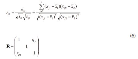
where the elements of the correlation matrix are given by rij. R is a square pxp matrix, where p is the number of variables. The diagonal elements of R are equal to one.
PCA is the systematic analysis of the covariance or correlation matrix. It can be shown that the eigenvalues are positive and the eigenvectors are orthogonal for both matrices.[6] The eigenvector equation for C is
Cui=λiui (7)
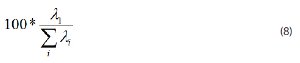
where ui is the ith eigenvector and λi is the corresponding eigenvalue. By convention the eigenvalues are placed in descending order, where λ1 is the largest eigenvalue. In PCA the eigenvectors are also called principal components. It can be shown that the 1st PC represents the largest source of variance in the data set. The percent variation explained by the ith PC is given by
It is common with spectral data that the data set can be well approximated by a few principal components. As explained earlier, score values provide information about the relationship between different observations. The PCs form a basis set which can be used to approximate the original data set. For a single mean-centered observation, xj,
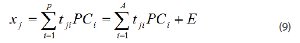
where tji are the score values, A is the number of principal components, E is the error when the number of principal components is less than the number of variables. Because the PCs are orthogonal, a direct expression for the score values can be given by the following equation.
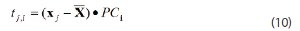
Equation 10 is derivable from equation 9 by taking a dot product of both sides and exploiting the orthogonality of the principal components.
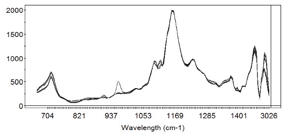
Figure 1-Mid IR spectra of a series of natural oils. The region between 1476 and 2997 cm-1 has been removed because it contains no relevant information for classification.
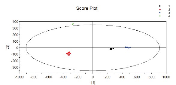
Figure 2- Score plot of mid IR spectral data for a series of oils. Legend group 1:corn oil, group 2: olive, group 3: safflower, group 4: corn margarine. The ellipse is the Hotelling T2 ellipse at 95% probability level. Samples outside the ellipse have a probability greater than 95% of being statistical outliers.
A common application of PCA on spectral data is a score plot. In a score plot, the scores of the samples for a pair of PCs are plotted. Score plots provide information about which samples are similar to each other, or what samples are possible outliers. Score plots can distinguish spectra that very similar using wavelength correlation analysis. For example Figures 1 and 2 shows the mid IR spectra and score plot for the mid IR spectra for a series of oils. Color coding the score plot clearly illustrates the differences between the four oils (olive, corn, safflower, and corn margarine). The samples that are farther away from the origin are more likely to be possible outliers. The ellipse in Figure 2 is called the Hotelling T2 ellipse and is showing the 95% probability level for outliers. The Hotelling T2 ellipse is based on scaled, squared score values [5]. The T2 value for observation i given.
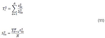
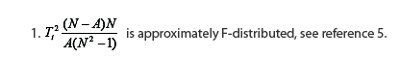
Where A is the number of principal components and tia is the ath principal component score value for the ith sample. T2 is closely related to the often used parameter Mahalanobis distance. An important property of the T2 statistic is that it is directly proportional to an F value, which is a statistical parameter that is rigorously related to a probability value.1 The numerical value of the F value is dependent on the number of samples, principal components, and probability level desired, α. Examination of equation 11 for two PCs shows that
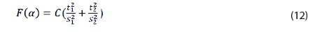
where C is a constant. Equation 12 is an equation for an ellipse in the t1, t2 space. By convention, the Hotelling T2 ellipse is usually drawn at the 95% probability level.
PCA can be viewed as a method for approximating the original data set. The approximation is based on a linear combination of the principle components where the amplitude coefficients are the previously described scores. The approximation is exact when the number of principle components equals the number of variables in the data set. For most spectral data sets, a small number of principle components (also called factors) can be used to approximate the spectral data set very well. The determination of the correct number of factors can be done by a variety of numerical methods. Too many factors in the PCA model will over fit the data and the model will not predict reliably. Most multivariate analysis software packages will suggest a suitable number of principle components. The suggested number is usually a good starting point; however, it is best practice to verify the optimum number of principle components with additional independent test data.
SIMCA
Classification is an important application of chemometrics. Classification is the sorting of data into different groups. In this section we will discuss soft independent modeling of class analogies (SIMCA) [7]. SIMCA is a method for classification of similar classes using multivariate analysis. SIMCA is a more sensitive improvement over PCA for group classification. PCA score plots sometimes show data sets to consist of several subgroups. For example Figure 2 shows the score plot for the mid IR spectra for a series of oils. Color coding the score plot clearly illustrates the differences between the four oils (olive, corn, safflower, and corn margarine).
SIMCA is designed to improve on the separation of classes obtained using PCA by using the residuals from the PCA. Residuals are the difference between the PCA model and the data. In the SIMCA analysis, a separate PCA model is built for each class in the training set. The average residual value for each class (S0) is also calculated. Test or validation data are then fit to each PCA class model. The correct class is the class which has the best fit to the PCA model. The comparison is quantified by the use of the scaled residual S0 (DmodX) values. The equations are given below
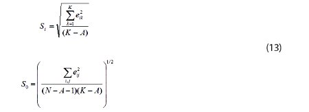
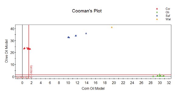
Figure 3- Cooman’s plot comparing the olive and corn oil classes using a test set. Legend circle: corn oil, diamond: olive oil, cross: safflower oil, triangle: walnut. See text for details.
N is the number of samples, A the number of principal components, K the number of variables, Si is the root mean square residual value for the ith sample, and eij is the spectral residual, i.e. the difference between the spectra and the PCA model for observation i and variable j. If the test sample residual is close to the average residual for the entire class, then the sample has a high probability of belonging to the class. The relationship to actual probability values is possible because the scaled residual values in equation 13 are described by an F-distribution. The results of a SIMCA analysis are often displayed in a Cooman’s plot. In a Cooman’s plot two classes are compared as shown in Figure 3.
A typical Cooman’s plot is shown in Figure3. PCA models for corn oil and olive oil are used to predict the classification of a set of test samples. The test samples include olive, corn, corn margarine, safflower and walnut oils. These test samples are distinct from the samples used to construct the SIMCA models. The different classes are color coded as shown in the legend. The x-axis on the Cooman’s plot is the DmodX (distance to model) value for the corn oil; the y-axis is the same for olive oil. The red vertical line is the 5% probability level for the corn oil model, samples to the right of this line are probable outliers for the corn oil models. The red vertical line is the same for olive oil. Note most olive and corn oil test samples are correctly classified. Test samples from other classes are well separated from the oil and corn oil groups. A walnut oil challenge sample is separate from the other four oils.
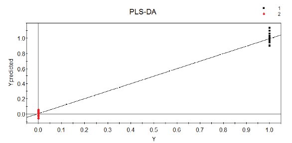
Figure 4- PLS-DA calibration curve for two classes of ascorbic acid measured with FT-NIR.
PLS-DA
Partial least squares-discriminate analysis (PLS-DA) is a very sensitive method qualitative classification method. PLS-DA is good method to try when SIMCA is not quite adequate to separate two very similar classes. In PLS-DA, each class is assigned an integer value (e.g. 0 or 1). The ordinary PLS algorithm is then applied with the class values as Y variables. A mathematical discussion of PLS regression can be found elsewhere [5,8]. Consider two forms of ascorbic acid measured using FT-NIR spectroscopy. The spectra for the two classes are nearly identical. SIMCA can be used to classify the data set, but the results are not optimum. A PLS-DA calibration curve is shown in Figure 4. PLS-DA successfully classifies this spectral data, using a four factor model.
Conclusion
This chapter has briefly summarized the use of chemometrics for the qualitative analysis of spectral data. In addition to quantitative analysis, there are many applications of chemometrics that have not been discussed here due to space limitations. Two important examples of this are chemical imaging and batch monitoring. Raman and NIR chemical imaging have been applied to pharmaceutical products including tablets [9] and drug coated stents [10]. Both Raman and NIR chemical imaging methods typically require chemometrics for the creation of useful images. Batch monitoring involves the use of multivariate control charts based on score plots developed from a collection of good batches [5,11]. Batch monitoring can be used with spectral or process data. Batch monitoring has been used to monitor a variety of complex pharmaceutical products to improve yields and provide improved process understanding [11]. In summary, chemometrics is a vital part of process analytical technology, quality by design, and the overall future of both pharmaceutical development and manufacturing.
References
- US Food and Drug Administration, Guidance for Industry Process Analytical Technology (2004)
- Siesler H, Ozaki Y, Kawata Y, Heise H Near-Infrared Spectroscopy: Principles, Instruments, Applications Wiley (2002)
- Long, F. Am. Pharm. Rev. Sept/Oct (2008)
- Long, F. “Vibrational Spectroscopic Methods for Quantitative Analysis”, in Handbook of Stability Testing in Pharmaceutical Development, K. Huynh-Ba (ed.), Springer 2009
- Eriksson L, Johansson E, Kettaneh-Wold N, Trygg J, Wikström, Wold S Multi- and Megavariate Data Analysis. Umetrics AB (2006)
- Strang, G. Computational Science and Engineering, Wellesley-Cambridge Press (2007)
- Wold, S. Pattern Recogn. Vol 8 (1976), pp. 127-139.
- Esbensen, K Multivariate Data Analysis- in practice. CAMO Process AS (2002)
- LaPlant, F. American Pharmaceutical Review, Vol 7, (2004) 16-25.
- Balss K, Long F, Veselov V, Akerman E, Papandreou G, Maryanoff C Anal Chemistry Vol 80 (2008) pp 4853-4859.
- Wold S, Cheney J, Kettaneh N, McCready C Chemometrics and Intelligent Lab Systems Vol 84 (2006) pp 159-163.
Author Biography
Dr. Frederick H. Long established Spectroscopic Solutions in the summer of 2001. Spectroscopic Solutions provides consulting and training in the areas of process analytical technology, spectroscopy, and statistics for regulated and non regulated industries. He received his S.B. and S.M. in Physics from the Massachusetts Institute of Technology and a Ph.D. in Chemical Physics from Columbia University.
This article was printed in the September/October 2011 issue of American Pharmaceutical Review - Volume 14, Issue 6. Copyright rests with the publisher. For more information about American Pharmaceutical Review and to read similar articles, visit www.americanpharmaceuticalreview.com and subscribe for free.