Robert Dream- HDR Co., LLC
The principal advantage of the three different filtration/separation techniques is that the operation is achieved without change or interphase transfer, thus any desired product is continually maintained in an aqueous environment. Size differences provide one basis on which the separations occur. The three available separations are Microfiltration (MF), Ultrafiltration (UF), and Nanofiltration (NF), respectively from large pore size retainment to smaller pore size retention. These techniques separate molecules of different sizes based on their size by retaining the larger size and permeating the smaller size. Product (mostly biologic) purification is broken down into four steps.
- First step is removal of insoluble
- Second step is isolation
- Third step is primary purification
- Fourth step is polishing or final purification
Microfiltration, Ultrafiltration and Nanofiltration
These three filtration types are similar in principle and operation but depending on the function they are used for there are subtle differences between them. Also, the pore size of the membranes is different. The microfiltration and nanofiltration operations are employed to concentrate products and/or switch carrier solvents. In this case, the retentate is the product. Usually, the ultrafiltration process is employed to purify products from suspended contaminants and permeate is the product. Microfiltration usually fits within the first category, ultrafiltration fits within the second and third categories, and nanofiltration fits within the fourth category.
Microfiltration retains particles 0.1-10 microns in diameter, for example, whole cells or cell debris. Common materials used for the manufacture of micro-filters include paper, polymers, and ceramics. In addition, most micro-porous membranes are symmetric or isotropic, that is, the membrane pores are the same size throughout the depth of the filter.
Ultrafiltration, which excludes particles and macromolecules of 1,000– 500,000 Dalton, is usually asymmetric or anisotropic. Anisotropic membranes consist of an extremely thin “skin” of homogeneous polymer supported upon a much thicker, spongy substructure. The pores of the skin layer are markedly smaller than the pores through the rest of the membrane. Consequently, the thin surface layer constitutes the major transport barrier and governs the filtration characteristics of the entire membrane.
Nanofiltration, is for the concentration of compounds with molecular weights of 250-2000 Daltons, and removing monovalent salts, methanol, and/or Ethanol from aqueous solutions of these compounds.
Analyzing Transmembrane Flux
During membrane separation processes, a set of feed pressure forces the solvent, and certain solutes, to flow through the membrane, while undesired solutes are retained, Figure 1.
To be effective the feed pressure must be greater than the osmotic or bulk pressure of the solution. For dilute solutions and with the pressure exerted on one side of the homogenous, isotropic membrane, the steady-state, transmembrane solvent flux can be approximated by the following relations;
The flux of the solute can be expressed by the following relation;
Where;
Jw = Solvent flux [cm3 (cm2 .s)]
Js = Solute flux [gm (cm2 .s)-1]
Lp = Membrane permeability for the solvent [cm3 (cm2 .s.atm)-1]
Ps = Membrane permeability for the solute (cm/s)
∆P = Hydrostatic pressure difference across the membrane (atm)
∆π = Osmotic pressure
σ = Reflection coefficient
∆C = Solute-concentration difference across the membrane (gm/cm3 )
[sometimes referred to as the solute-concentration difference between the upstream and downstream solutions]
C̄= Average concentration of solute in the upstream solution
(1-σ) = the quantity represents the fraction of the solvent flux carried by pores large enough to pass the solute
If the reflection coefficient (σ) is small (σ≅ 0), the membrane will be highly permeable to both solute and solvent; if σ is large (σ≅ 1), the membrane will reject all solute.
The first term on the right-hand side of equation (2), corresponds to the diffusive flux of solute through the membrane. The second term represents the “convective flux” or “coupled transport” of solute driven by the net flux of solvent (it is sometimes interpreted as a consequence of frictional drag between moving solvent molecules and solute molecules within the membrane). In addition, a high diffusive flux of solvent will result in momentum exchange between solvent and solute molecules, due to collisions, which could serve to increase the net flux of solute. Such momentum interchange would not be expected to cause a significant reduction in the diffusive flux of the more abundant solvent molecules, however, no term accounting for coupled transport is included in equation (1).
From mass conservation, the solute flux, Js , can also be written in the form,
Where Cperm is the concentration of permeate or ultrafiltrate (the concentration in the downstream solution), and Jv , is the total flux of permeate (usually assumed to be equal Jw for dilute solutions). Alternatively, Js can be expressed in terms of C∞, the concentration of solute in the upstream solution:
Where R is the rejection coefficient, which is equal to the fraction of solute present in the upstream solution that is rejected by the membrane. In terms of concentrations, the rejection coefficient is defined as;
Finally, we should note that for a purely diffusive-type membrane (for which Jw is negligible), the solute mass flux is;
Where Ks is the distribution coefficient of solute between the membrane and solution (assumed to be constant), De is the effective diffusivity of solute through the membrane, and δ is the membrane thickness. Equation (6) models the membrane as a continuous “solvent” in which the solubility of solute is described by the distribution coefficient Ks. An alternative approach is to treat the membrane as a sieve with distinct pores and a specific porosity.
Concentration Polarization
During the concentration of the feed, pressure exerted on the upstream solution in contact with the membrane causes solute to flow toward the membrane surface. Initially, the convective flux of solute to the membrane exceeds the rate at which solute passes through the membrane, this results in the accumulation of solute at the membrane, with the maximum solute level at the membrane surface. Such phenomenon is known as concentration polarization, Figure 2.
If the membrane is not completely impermeable to the solute, such polarization can cause solute leakage through the membrane, or anomalously low reflection efficiency. In addition, the high concentrations of solute can increase the osmotic pressure difference (i.e., the pressure difference across the membrane wall), and thus reduce the effective driving force for solvent transport through the membrane. In many cases particularly with macromolecular solutes, concentration polarization is the limiting factor governing flux rates.
Concentration polarization is often unavoidable but should be minimized. In practice, a nitrogen pulse or other method is supplied on the permeate side of the membrane, creating a shock wave that causes accumulated solute to dislodge from the feed side of the membrane and become part of the retentate stream, Figure 2.
During this activity, the permeate valve will be closed. Cross-flow filtration or vigorous mechanical stirring of the upstream liquid is also employed to alleviate the effects of concentration polarization.
Gel Polarization
If the concentration of solute at the membrane surface is high enough, the polarization layer exhibits gel-like properties. At this point, gel[1]polarization is said to occur. The layer of concentrate assumes the form of slime or cake at the membrane’s surface, and the adherent layer presents a hydraulic barrier in series with the membrane. In fact, the gel (when present) usually contributes the dominant resistance to mass flow.
The concentration of solute at which gel filtration takes place will vary with the size, shape, and degree of the solvation of the solute particles.
For proteins and nucleic acids, concentrations as high as 10-30 percent by weight are often required before gelation is observed. In contrast, with rigid-chain, solvated macromolecules like polysaccharides, a concentration below 1% by weight may be sufficient.
Effects of Polarization
To analyze the effects of polarization on solvent flux, we recall that the volumetric flux of solvent, Jw, can be written as;
And;
Where the osmotic pressure, Δπ, has been expressed in terms of Cwall, the concentration of solute at the surface of the membrane. Integration of a steady-state mass balance on solute in the polarization layer leads to;
Where Ds is the diffusivity of solute (assumed here to be independent of solute concentration).
Furthermore, if σ=1, that is, if Cperm=0, then;
This equation provides a relationship between the boundary layer thickness, δ, and the concentration of solute at the membrane surface, Cwall. Note that if gel polarization occurs, Cwall = Cg , the gel concentration of the macrosolute. The gel concentration of course places an upper limit on the solute concentration at the membrane surface.
At this point we should consider another subtle yet important distinction between concentration polarization and gel polarization. In the former, Cwall is less than Cg , and Cwall/C∞ will adjust itself to an imposed Jw. Nonetheless, the polarized region presets a resistance to mass transfer and can be modeled as a membrane in series with original membrane. The resulting flux is given by
Where (1/Lp ) is again the membrane resistance Rp is the resistance of the polarized boundary layer. Increasing the transmembrane pressure drop will increase c0s and consequently, Rp . Thus; concentration polarization causes the flux, Jw, to increase less than proportionately with ΔP. On the other hand, gel polarization results in a constant value of Cwall = Cg . Equation (10) then predicts that the flux will be independent of the applied pressure. Such behavior has indeed been observed for many systems, particularly at high pressures.
Returning to equation (10) the leading terms on the right-hand side, Ds /δ, can be viewed as a mass transfer coefficient, ks , which allows us to write;
Mass transfer coefficients for fluid flow in narrow channels conventionally are described by expressions of the form;
Where;
dh = Equivalent diameter of the channel, or
dh = 4(Cross-sectional area / wetted perimeter)
u = Average velocity of the fluid along the channel
ρ = Density of the fluid
μ = Viscosity of the fluid
Re = Reynolds Number
Sc = Schmidt number
And, A and a are constants.
Time Required for Ultrafiltration
Suppose we wish to concentrate a protein solution by ultrafiltration in a batch system. The permeability of the membrane is Lp liter m-2hr-1atm-1, and the total membrane area is A m2 . The initial volume of solution is V0 liter and the amount of protein present is n1 mmoles. The pressure drop is ΔP atm and the temperature of operation is T°K assuming that the membrane completely rejects the solute and that concentration polarization is negligible.
a. Derive an expression for the rate of change of the batch retentate volume with time (dV/dt).
b. Derive an expression for the time required for ultrafiltration of the solution (reduce the volume from V0 liter to V liter).
Solution:
a. In our analysis of ultrafiltration, we would most like to have the time required to filter a given volume of feed. To find this time we first must find the solvent velocity through the membrane. This velocity is given by equation (1)
If the solute is completely rejected by the membrane, the reflection coefficient σ=1; if the solution is dilute, the osmotic pressure Δπ=RTCwall, where Cwall is the solute concentration at the surface of the membrane.
But what is Cwall? If the mixing in the holding tank were complete, then the concentration at the membrane surface Cwall should equal the concentration in the tank C∞. However, mixing is incomplete and these concentrations are not equal. Instead, the concentration at the membrane’s surface may be much more than that in the bulk because the solvent flux through the wall strands solute near the wall. This high solute concentration, called concentration polarization, is illustrated schematically in Figure 3. It augments the osmotic pressure and, hence, reduces the flux through the membrane. To estimate this flux reduction, we recognize that solute carried toward the membrane by solvent convection must equal that diffusing away from the wall by diffusion:
This differential equation is subject to the boundary conditions that at the wall, the concentration is Cwall-Cperm:
and at,
Where δ is the thickness of a thin layer near the surface.
Solving first order differential equation (15) and applying boundary conditions (16) and (17),
Furthermore, if σ=1, that is, if Cperm=0, then
In other words, a plot of flux versus the logarithm of reservoir concentration C∞ should be a straight line.
The variation of flux with reservoir concentration suggested by equation (18) can be checked experimentally. The small scatter in these data is typically of the success of the analysis. Note that the slope of this plot equal to (-De/δ), is a type of mass transfer coefficient.
Now we return to our original goal of estimating the time required to filter a given volume. In general, this analysis is complicated, involving transcendental equations. The most useful simple case occurs when there is little concentration polarization, that is, when
In this case, Cwall = C∞.
We now make a mass balance on the solvent and combine the result with equation (1):
Because the membrane rejects all the solute, the total solute (n1 = C∞V) is constant and equation (21) becomes:
b. This equation is easily integrated using the initial condition
Examples
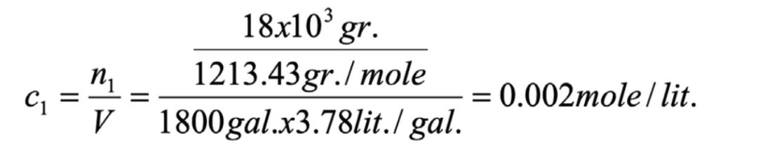
Example 1: We wish to concentrate and achieve a solvent switch of a solution by cross-flow microfiltration in a batch system. The flux for this ceramic membrane is 10 gal/hr-ft2 . The initial volume of the solution is 1800 gal and the final volume is 360 gal, the amount of protein present is 18.0 Kg, and the molecular weight is 1213.43 gr./ mole. The pressure drop is 30 psig and the temperature of operation is 277°K. If we want the operation to be completed in 2 hours calculate the required area to achieve this task.
Solution:
R=0.082-liter atm/gr.mole°K
T=277°K
n1 =(18x103 gr/1213.43 gr./mole)
Δp=30 psig
V0 = 1800 gal
V = 360 gal
t = 2 hrs, assumed
j v = 10 gal/hr-ft2
The time required for Micro-filtration is;
Then the term,
and from equation (1), the term,
can be calculated;
Therefore equation (1) reduces to;
Also;
But;
or
Substituting;
Rearranging equation (1);
And the term is a small value, therefore from equation (2) we have.
then equation (3) reduces to:
or
And therefore;
A= 68.18 ft2 , is the area required to cross flow 1800 gal. to 360 gal in two hours.
Example 2: If we assume that the membrane completely rejects the solute and that concentration polarization is negligible, then repeat example 1.
Solution:
V0 = 1800gal
V =360 gal
t = 2 hrs
j v =10 gal/hr-ft2
R=0.082 lit.atm/gr.mole.°K
T=277°K
n1 =(18x103 gr./1213.43gr./mole)
Δp=30 psig
MW=1213.43
The time required for Micro-filtration is;
If we assume the term,
Is small, then equation 1, reduces to:
Assume the term is small, then:
Because,
And n1 = c1 V.
Then equation (1) reduces to;
Or
And therefore;
A= 72 ft2 .
Example 3: We wish to concentrate and achieve a solvent switch of a solution by cross-flow Nano-filtration in a batch system. The flux for this membrane is 5 gal/hr-ft2 . The initial volume of the solution is 667 gal and the final volume is 119 gal, the amounts of protein present is 18.0 Kg, and the molecular weight is 1213.43 gr./mole. The pressure drop is 400 psi and the temperature of operation is 277°K. If we want the operation to be completed in 2 hours calculate the required area to achieve this task.
Solution:
R=0.082 lit.atm/gr.mole°K
T=277°K
n1 =(18x103 gr/1213.43 gr./mole)
Δp=400 psig
V0 = 667 gal
V = 119 gal
t = 2 hrs, assumed
j v = 5 gal/hr-ft2
The time required for Nano-filtration is;
Then the term,
and from equation (1), the term,
can be calculated;
Therefore equation (1) reduces to;
Also;
But, n1 = c1 V
Or
Substituting;
Rearranging equation (1);
And the term (RTc1/ΔP) is a small value, therefore from equation (2) we have.
Then equation (3) reduces to:
and therefore;
A= 54.23 ft2 , is the area required to cross flow 667 gal. to 119 gal in two hours.
Example 4: If we assume that the membrane completely rejects the solute and that concentration polarization is negligible, then repeat example 3.
Solution:
V0 = 667 gal
V =119 gal
t = 2 hrs
j v =5 gal/hr-ft2
R=0.082 lit.atm/gr.mole. °K
T=277°K
n1 =(18x103 gr./1213.43gr./mole)
Δp=400 psig
MW=1213.43
The time required for Nano-filtration is;
If we assume the term,
Is small, then equation 1, reduces to
Assume the term (RTc1/ΔP) is small, then:
Because,
And n1 = c1 V.
Then equation (1) reduces to;
Or
And therefore;
A= 54.8 ft2 .
System Data Digitization of the Input/ Output Hierarchy
Digitalization of any manufacturing industry is a key step in any progress of the production process. The process of digitalization includes both increased use of robotics, automatization solutions, and computerization, thereby allowing to reduce costs, to improve efficiency and productivity, and to be flexible to changes. The biopharmaceutical industry has however been resistant to digitalization, mainly due to fair experience and the complexity of the entailed development and manufacturing processes. Nevertheless, there is a clear need to digitalize as the demand for both traditional and new drugs is constantly growing.
![Figure 4. The evolution of process development, from one-factor-
at-a-time (OFAT), through design of experiments (DoE), to high-throughput process development (HTPD), raw material insights and quality by design (QbD), and now mechanistic modeling [2].](http://media.americanpharmaceuticalreview.com/m/28/article/609734-4.jpg)
An exponential progress and growth in innovation and development of new technologies today have reached new heights in creating and implanting digital platforms, e.g.; PAT (process analytical technology), QbD (quality by design), digital sensor, IIoT (industrial internet of things), and AI (artificial intelligence) are few to note that creating a paradigm shift and acceptance by industry and regulatory.
Today we can avoid all the manual equation solving, data manipulations, and the tedious effort to qualify the obtained results by using statistical models. We can use input/output models by using mechanistic models to gain the same results. By developing unit models starting from process development through clinical and product launch (throughout the lifecycle), figure 4. Mechanistic modeling has evolved from the following steps; studying one-factor-at-a-time (OFAT), design of experiments (DoE), high-throughput process development (HTPD), raw material insights and quality by design (QbD), platform knowledge, and mechanistic modeling.
Since mechanistic models are based on natural laws, they are valid far beyond the calibration space. In practice, this means that the process setup and parameters can easily be changed. Such as switching and changing from batch to continuous processing, changing type, size, dimensions, and much more. As the parameters (CMAs, CPPs, CQAs) are based on natural principles, mechanistic models allow you to generate mechanistic process understanding and thus fulfill QbD obligations (ICH Q8), which is not the case with statistical models.
- This opens a wide range of applications using the same mechanistic model without any further experimentation, including early-stage process development, process characterization and validation, and process monitoring and control.
- Even completely different scenarios can be simulated with no additional experimental effort, such as overloaded conditions, flow-through operations, or continuous filtration.
- The model will evolve with the proceeding development lifecycle and account for holistic knowledge management, enabling a fast and lower-cost replacement of lab experiments with computer simulation.
A mechanistic model is a type of model that assumes a complex system can be understood by examining the workings of its individual parts and the manner in which they are coupled. Mechanistic models are typically based on mathematical descriptions of mechanical, chemical, biological, or other phenomenon or processes. A good example of a mechanistic model is the propagation of sound in random media, which can be described by stochastic differential equations.
A digital processor to perform numerical calculations on sampled values of the signal, figure 5.
The processor may be a general-purpose computer such as PC, or a specialized DSP (Digital Signal Processor) chip. The analog input signal must first be sampled and digitized using an ADC (analog to digital converter).
Digitalization of any manufacturing industry is a key step in any progress of the production process. The process of digitalization includes both increased use of robotics, automation solutions and computerization, thereby allowing to reduce costs, save time, to improve efficiency and productivity, and to be flexible to changes. To implement digitization it is required to plan, digitization planning/process of a manufacturing operation in the biopharmaceutical industry (Figure 6).
GMP Planning and Implementation
Digitization and data harness are new sources of data, fed into systems powered by machine learning (ML) and Artificial Intelligence (AI), are at the heart of this transformation. The information flowing through the physical world and the global economy is staggering in scope. It comes from thousands of sources: sensors, satellite imagery, web traffic, digital apps, videos, and credit card transactions, just to name a few. These types of data can transform decision-making. In the past, a packaged food company, for example, might have relied on surveys and focus groups to develop new products. Now it can turn to sources like social media, transaction data, search data, and foot traffic; all of which might reveal that Americans have developed a taste for Korean barbecue, and that’s where the company should concentrate.

The US Food and Drug Administration (FDA) now has many guidelines for GMP in the biopharmaceutical business, which cover process validation and data integrity. The FDA defines current GMP as systems that provide proper design, monitoring, and control over manufacturing processes and facilities in the pharmaceutical industry. These systems are intended to assist organizations in ensuring the identification, strength, purity, and quality of drug substance and products.
In other regulatory bodies, e.g., GMP inspections are carried out by National Regulatory Agencies within the European Union, the European Medicines Agency (EMA) oversees inspections to ensure that these standards are followed and are significant players in standardizing GMP activities across European Union (EU). GMP must be followed by any manufacturer of pharmaceuticals for the EU market, regardless of where they are based in the world. The Health Products and Food Branch Inspectorate oversee GMPs in Canada, while the Medicines and Healthcare Products Regulatory Agency (MHRA) in the United Kingdom conducts GMP inspections. Routine GMP inspections are conducted by each inspectorate to guarantee that drug items are manufactured safely and correctly. In addition, many national bodies across the world conduct routine GMP inspections to verify that drug products are manufactured safely and correctly. Many countries also conduct pre-approval inspections (PAI) for GMP compliance before the marketing authorization of a new medicine. The digitization and digital data collection will streamline the inspection and review process and improve record keeping that is required by the regulatory. It will assist in CAPA and OOS investigation as well.
There are challenges and opportunities in the digitization of drug product operation and manufacture, Figure 7 depict a summary outline of these opportunities and challenges.
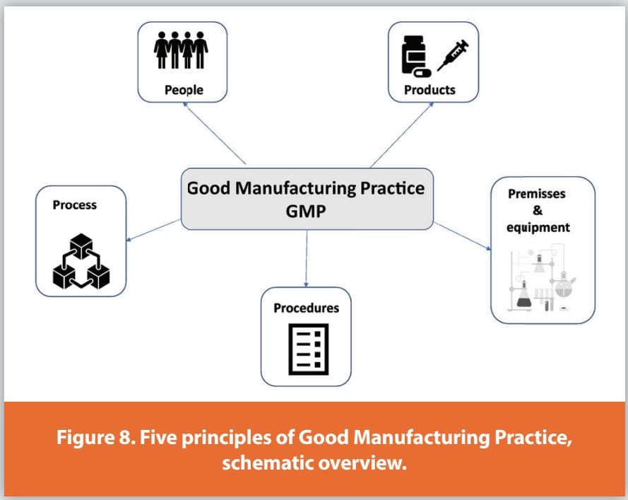
Regulations allow medicine, medical device, food, and blood products, processors, and packagers to take proactive actions to guarantee that their goods are safe and effective. GMP regulations, codes and standards demand quality-oriented approach, risk-based validated drug product manufacturing. Allowing businesses to reduce or eliminate contamination, mix-ups, and errors, figure 8 depict simplified look at the requirement.
References
1. Robert Dream, “How to Design Nano-, Ultra-, and Microfiltration Systems”, Chemical Engineering Journal, January 2000.
2. Mechanistic modeling of chromatography: opportunities and challenges, Cytiva. Chromatography mechanistic modeling | Cytiva (cytivalifesciences.com)
Publication Detail
This article appeared in American Pharmaceutical Review:
Vol. 26, No. 8
Nov/Dec 2023
Pages: 8-17
Subscribe to our e-Newsletters
Stay up to date with the latest news, articles, and events. Plus, get special
offers from American Pharmaceutical Review delivered to your inbox!
Sign up now!